CPU vs GPU Distributed Computing — Two Engineering Implementations of the Same BSP Theory
In Spark, reduceByKey aggregates key-value pairs scattered across dozens of machines — a single call takes milliseconds to seconds; in PyTorch DDP training, the NCCL AllReduce triggered by loss.backward() sums gradients across thousands of GPUs — a single call takes tens of microseconds. The two operations have nearly identical names but differ by two to three orders of magnitude in practice. Yet the more paradoxical thing is: their core math is exactly the same.
This isn’t coincidence — it’s common descent. The vocabulary was set in stone back in the MPI standard of 1994 — MPI_Reduce, MPI_AllReduce, MPI_Bcast, MPI_AllGather, MPI_Alltoall. Over 30 years these primitives evolved along two branches: one entered the world of cheap fault-tolerant commodity clusters like Hadoop/Spark, the other entered the world of tightly-coupled HPC / GPU training like MPI/NCCL. The theory is fully unified, but the engineering constraints are radically different — fault-tolerance strategy, communication granularity, sync frequency, programming model, hardware interconnect, every item differs by one or two orders of magnitude.
This article walks a single thread comparing the two worlds — same math, two engineering implementations. Once you understand at this level, Spark’s shuffle and NCCL’s AllReduce become two constraint-specific implementations of the same thing; cross-domain knowledge transfer (from Spark engineer to distributed ML engineer) becomes exponentially cheaper — because the cognitive framework is already built.
Common Ancestor — MPI 1994 · BSP 1990
Why does the vocabulary overlap? Because both streams flow from two common sources: the BSP (Bulk Synchronous Parallel) model and the MPI (Message Passing Interface) standard. The former is a theoretical parallel computing model proposed by Leslie Valiant in 1990, abstracting all parallel algorithms as cyclic supersteps of “local compute → communication → global synchronization”; the latter is a parallel programming interface standard set in 1994, defining a set of collective communication primitives. BSP provided the theoretical framework, MPI provided the API names, and together they shaped every large-scale parallel computing system of the past 30 years.
This tree resolves the first puzzle — why Spark and NCCL share terms like reduce / allreduce / broadcast / gather. They all stem from MPI; MPI defined a standardized set of “collective communication primitives,” and subsequently every cheap cluster, supercomputer, or GPU training framework reused this vocabulary.
But this tree also seeds the second puzzle — if the terms are the same, why are the implementations so far apart? The answer lies in the engineering constraints at each branch — when Hadoop ported MPI ideas to “tens of thousands of cheap machines, with several failing every day,” fault tolerance became the top priority; when NCCL ported MPI ideas to “8 GPUs fully interconnected via NVLink, each step measured in tens of microseconds,” peak bandwidth became the top priority. The constraints diverge completely, so engineering implementations diverge naturally.
BSP Model — Local Compute → Communication → Global Sync
Draw all the above systems on a single chart and you can immediately see how the BSP model unifies them:
Lay these four systems side by side in the BSP framework and the differences become immediately clear — the three-stage skeleton is identical, the absolute timings differ by several orders of magnitude. This is the essence of “same BSP theory, different engineering constraints.” A PyTorch DDP step takes about a millisecond, a Spark stage about a minute — three orders of magnitude apart, yet both follow the cycle of “local compute → communication → global sync → next superstep.”
This explains why the vocabularies of these two domains overlap — structurally they are the same thing; only the specific parameters (latency, bandwidth, fault tolerance, granularity) differ.
”Distributed” Inside a Single Machine — CPU OOO Engine vs GPU Warp Scheduler
The word “distributed” isn’t only for multi-machine — how multiple execution units cooperate inside a single machine is the same class of problem. Here the CPU and GPU design philosophies are diametrically opposed: CPUs hide all scheduling complexity inside hardware, while GPUs simplify scheduling to the extreme and hide latency through massive parallelism.
| Dimension | CPU OOO Engine | GPU Warp Scheduler |
|---|---|---|
| Branch Predictor | Modern CPUs achieve 95%+ accuracy; misprediction rolls back tens of cycles | None. Divergent branches within a warp serialize via warp divergence |
| Reorder Buffer (ROB) | Intel Golden Cove has 512 entries to extract deep parallelism | None. Each warp executes strictly in-order |
| Reservation Station | Complex dependency tracking + port allocation | Minimal. Just picks “warps with operands ready” to dispatch |
| Register Renaming | Hundreds of physical registers to eliminate false dependencies | None. Each warp has its own physical register allocation |
| Speculative Execution | Predicts and runs ahead on the predicted path | None |
| Memory latency hiding | ILP within a single thread; OOO covers hundreds of cycles | Switch to another warp; up to 64 warps available per SM |
| Silicon area for scheduling | ~50% of the core | ~10%, with 90% dedicated to execution units |
A CPU core devotes 50% of its silicon to scheduling, leaving the ALUs that actually do work as a minority. The GPU SM is the opposite — scheduling takes only a small corner, with the bulk of the area given to execution units like CUDA core / Tensor Core / SFU / TMA. That’s why on the same silicon area, GPU AI throughput is tens to hundreds of times that of a CPU — it reclaims all the scheduling area and packs in ALUs.
The fundamental opposition in design philosophy can be summed up in one sentence:
CPUs solve “make single-threaded code fast” — only so much parallelism is available within a single program, so complex hardware extracts every last drop of ILP. GPUs solve “lots of threads is fast” — hardware never lacks independent instructions (the next one comes from another warp), so scheduling stays minimal.
This pair of philosophies determines every other design decision on both sides — from memory hierarchy to execution units to programming model, all flow from this main thread.
Memory and Data Movement — Implicit Cache+DMA vs Explicit SMEM+TMA
The second fundamental difference between the two worlds’ “in-machine distribution” — CPUs let you forget the memory hierarchy; GPUs force you to face it head-on.
In the CPU world, almost everything about memory is implicit:
- Multi-level cache (L1/L2/L3) is fully automatic — when you write
int x = arr[i], hardware automatically decides which level the data comes from and when to evict. - Hardware prefetcher — the CPU proactively guesses your next access and fetches ahead. Modern CPUs run 4-5 prefetchers in parallel.
- DMA controller — bulk data transfer (disk / NIC / memory-to-memory) is handled by DMA; the CPU just configures and continues.
- OOO execution hides memory latency — a load takes 100 cycles, the CPU immediately runs unrelated subsequent instructions.
GPUs take the opposite approach:
- Explicit hierarchy —
__shared__/__constant__/ registers / global memory, the programmer must explicitly choose where data goes. - Explicit asynchronous transfers —
cuda::memcpy_async, TMA descriptors,cp.asyncPTX instructions; data doesn’t move from GMEM to SMEM by itself. - Explicit synchronization —
__syncthreads()waits on all threads; async barriers wait on a specified number of bytes. - Software prefetch — no hardware prefetcher; instead, double-buffering — the programmer writes code so that “while computing the current tile, TMA asynchronously fetches the next tile.”
Lay the comparison side by side:
| Function | CPU Solution | GPU Counterpart | Control Mode |
|---|---|---|---|
| Cache recent accesses | multi-level cache, automatic | L1 / L2 + SMEM | CPU automatic, GPU semi-manual |
| Bulk data transfer | DMA controller (peripheral ↔ memory) | TMA (GMEM ↔ SMEM) | both require configuration |
| Predict next access | Hardware Prefetcher | none · software double-buffer | CPU hardware / GPU software |
| Hide memory latency | OOO + speculation | warp switching | CPU intra-thread ILP / GPU thread switching |
| Memory hierarchy choice | transparent (cache automatic) | explicit (__shared__ etc.) | CPU implicit / GPU explicit |
| Cross-device transfer | DMA + system bus | NVLink + GPUDirect | similar in concept, GPU much faster |
The most interesting correspondence is DMA and TMA: the concept is consistent — offload data movement to dedicated circuitry so the general-purpose compute units don’t waste cycles on repetitive work. The differences are:
- DMA: external to the CPU, cross-device transfer, large granularity (whole files), CPU triggers occasionally.
- TMA: inside the SM, transfers within the on-chip memory hierarchy, tensor-structured (multi-dimensional), single-thread frequent invocation.
Why does the GPU put a “DMA” inside the SM? Because Tensor Cores are so fast that moving data becomes the first bottleneck. Putting move hardware right next to the compute units minimizes the overhead of transfer instructions. CPU DMA is designed for “occasional bulk transfers”; GPU TMA is designed for “sustained high-speed feeding” — the same idea landing in two different time scales.
The philosophical difference in one sentence:
The CPU tries to let you forget the memory hierarchy (automatic management); the GPU forces you to face it (manual optimization).
This is why CPU code “runs decently with little tuning,” while GPU code “can be 10-100× slower without optimization” — GPU explicitly hands the responsibility for performance tuning to the programmer, but as compensation, it dedicates every hardware resource to execution, so its theoretical peak is much higher.
Six Collective Communication Primitives — Broadcast · Reduce · AllReduce · AllGather · ReduceScatter · AlltoAll
Zoom from in-machine back to multi-machine distributed — collective communication primitives are the concrete operations of BSP’s communication phase. This set is defined in MPI, implemented as GPU versions in NCCL, and offered under different names in Spark. The six diagrams below are the “atomic operations” of distributed systems; any complex operation is a composition of them:
This table is the most direct evidence — each row is the same mathematical operation expressed through different interfaces in three worlds. Spark’s shuffle is essentially AlltoAll; MapReduce’s reduce phase is essentially Reduce; PyTorch DDP’s gradient sync is essentially AllReduce; FSDP’s parameter gathering is a composition of AllGather + ReduceScatter.
The engineering implementations focus on different details — Spark cares about how shuffle spills to disk, how it stays fault-tolerant, how to partition; NCCL cares about whether AllReduce uses Ring or Tree, how to exploit NVLink topology, how to overlap compute and communication. But they solve the same abstract problem class.
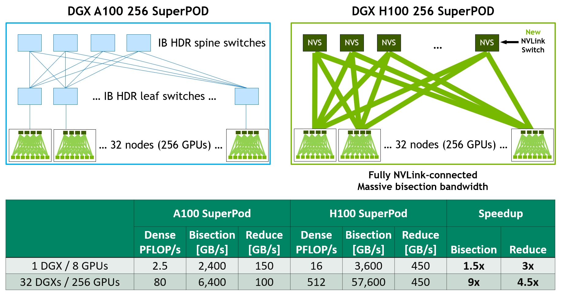
Communication Hardware Layer — PCIe vs NVLink/NVSwitch · Ethernet vs InfiniBand
Collective communication primitives run on top of communication hardware. This layer differs dramatically between the GPU and CPU worlds, primarily in bandwidth and latency.
| Interconnect | Per-link Bandwidth | Latency | Topology | Use Case |
|---|---|---|---|---|
| PCIe 5.0 | 64 GB/s | ~1 μs | shared bus | CPU ↔ GPU · CPU ↔ NIC |
| NVLink 5 (B200) | 1.8 TB/s/GPU | ~1 μs | point-to-point | GPU ↔ GPU in-machine |
| NVSwitch | full bandwidth | ~1 μs | all-to-all | DGX/NVL72 rack |
| NVLink-C2C | 900 GB/s | ~ns | point-to-point | Grace ↔ Hopper/Blackwell |
| InfiniBand HDR/NDR | 200-400 Gbps | ~1 μs | Fat-Tree | HPC + AI cross-machine |
| ConnectX-7/8 | 400-800 Gbps | ~1-2 μs | RDMA | NIC, cross-machine RDMA |
| Spectrum-X | 800 Gbps | ~2 μs | enhanced Ethernet | ”AI-optimized Ethernet” |
| Ethernet (commodity) | 10-100 Gbps | ~5-50 μs | TCP/IP | general data center |
Note: in the same rack, GPU-to-GPU bandwidth (NVLink) is ~1.8 TB/s, about 28× faster than PCIe 5.0 (64 GB/s). This is the essence of the difference between “NVLink domain” and “PCIe domain” — Tensor Parallel (frequent communication) is feasible inside the NVLink domain, but completely impractical across PCIe.
GPUDirect RDMA deserves a special mention. Traditionally, sending data from GPU 1 to GPU 2 (on a different machine) requires GPU 1 → CPU 1 memory → NIC → wire → NIC → CPU 2 memory → GPU 2, four memory copies. GPUDirect RDMA lets the NIC read directly from GPU 1’s HBM and write directly to GPU 2’s HBM, bypassing both CPUs’ memory, reducing to GPU 1 → NIC → wire → NIC → GPU 2, zero CPU memory copies. The savings are not just bandwidth but also CPU scheduling overhead — in large-scale training, the CPU becomes pure bystander.
The CPU distributed world has essentially no need for such “bypass-the-CPU” tricks — because communication granularity is naturally large, a few extra memory copies don’t matter against a seconds-long shuffle. In GPU training, each step is tens of microseconds, so any extra memory copy drags down the whole, which is why aggressive techniques like GPUDirect exist.
Communication Software Layer — NCCL · NVSHMEM · MPI · Hadoop RPC
Above the hardware sits the communication software library. In the GPU world, NCCL is the de facto standard; nearly every distributed AI training framework uses it as a backend. In the CPU world, MPI dominates HPC, and Hadoop/Spark use their own RPC frameworks.
| Library | Granularity | Sync Semantics | Fault Tolerance | Used by |
|---|---|---|---|---|
| MPI (OpenMPI / MPICH) | medium-coarse (KB-MB) | async, explicit Wait | almost none | HPC supercomputing + early ML |
| NCCL | medium (MB-GB) | async stream | only rudimentary in NCCL 2.20+ | all GPU training frameworks |
| NVSHMEM | fine (a few bytes) | one-sided, callable inside kernels | none | MoE training / custom high-performance kernels |
| GPUDirect RDMA | arbitrary | async | RDMA NIC’s own | NCCL uses automatically · engineers don’t touch directly |
| Hadoop RPC | coarse (GB-TB) | sync + async | strong · auto-recompute on node failure | Hadoop ecosystem |
| Spark RPC (Netty) | coarse | sync | strong · RDD lineage recompute | Spark ecosystem |
| gRPC / Akka | flexible | sync / async | depends on user | microservices / data platforms |
The most interesting comparison is between NCCL and NVSHMEM:
- NCCL is at “collective communication” granularity — a single
ncclAllReducecall synchronizes all GPUs, suitable for large data blocks. PyTorch DDP / FSDP / Megatron all use this granularity. It auto-detects topology (NVLink / IB / PCIe), auto-selects the optimal transport path, auto-uses tree for small messages and ring for large ones. - NVSHMEM is at “one-sided communication” granularity — one GPU directly reads/writes another GPU’s memory without the remote side’s involvement, and can be invoked from inside a CUDA kernel.
// NVSHMEM sends directly from inside a kernel
__global__ void custom_kernel() {
    if (threadIdx.x == 0) {
        nvshmem_float_p(remote_ptr, value, target_pe);  // 1 thread sends 1 float
    }
}
This fine granularity suits MoE routing (each token must go to the GPU hosting the right expert) and custom attention (frequent small-block KV exchange between GPUs). DeepSeek’s DeepEP library uses NVSHMEM to address MoE communication bottlenecks; FlashInfer also uses it extensively. There’s no counterpart at this granularity in the CPU distributed world — CPU communication overheads are simply too high for “send a message from inside a kernel” to be remotely feasible.
NCCL does an enormous amount of work behind a single ncclAllReduce call:
- Topology detection at startup (NVLink / IB / PCIe interconnect structure)
- Auto-selection of optimal transport (NVLink in-machine, IB + GPUDirect RDMA across machines, Ethernet + TCP without IB)
- Auto-selection of optimal algorithm (Ring AllReduce for bandwidth, Tree AllReduce for latency, Double Binary Tree for balance)
- Overlapping compute and communication (all NCCL APIs are asynchronous, running on a CUDA stream)
This whole automation pipeline lets a single loss.backward() in PyTorch DDP achieve near-optimal communication performance on any machine — the programmer doesn’t need to understand the hardware topology.
Four Generations of Distributed Training Frameworks — Horovod → DDP → FSDP → Megatron-Core
Above the communication library sits the distributed training framework. The past 7 years cleanly split into four generations by “which bottleneck did each solve”:
First generation (2017-2019) · Naive Data Parallel
- Horovod (Uber 2017) — ported Ring AllReduce from MPI into deep learning. Proved a path beyond the parameter server (PS). Discontinued (the Linux Foundation took over, but official maintenance has ceased); its ideas live on in PyTorch DDP.
- PyTorch DDP (2018) — today’s de facto standard.
loss.backward()automatically AllReduces gradients and overlaps compute and communication. - tf.distribute (built into TensorFlow) — Google’s in-house solution, mainstream for TPU users.
DDP’s limitation — each GPU must fit the entire model. 70B models can’t (parameters + gradients + optimizer state ~ 130 GB).
Second generation (2019-2021) · Memory-optimized Data Parallel
- DeepSpeed ZeRO (Microsoft 2019) — revolutionary “Zero Redundancy Optimizer.” Three stages:
- ZeRO-1: shard optimizer state (4× savings)
- ZeRO-2: + shard gradients (8× savings)
- ZeRO-3: + shard parameters (N× savings, more communication)
- FairScale (Meta 2020) — ZeRO experiment on PyTorch, deprecated, all features merged into PyTorch FSDP.
- PyTorch FSDP (2022) — official version of ZeRO-3. FSDP2 (2024) rewritten on DTensor, more advanced.
ZeRO’s memory optimization summary:
| Stage | Sharded objects | Memory savings | Communication cost |
|---|---|---|---|
| ZeRO-1 | optimizer state | 4× | same as DDP |
| ZeRO-2 | + gradients | 8× | slightly more |
| ZeRO-3 | + parameters | N× | significantly more (needs AllGather to temporarily collect) |
| ZeRO-Infinity | + CPU/NVMe offload | nearly unlimited | offload communication added |
Third generation (2021-2023) · 3D Parallel
Data Parallel + ZeRO only solves the “fits in memory” problem. When models exceed tens of billions of parameters and training compute requires thousands of GPUs, communication overhead in pure data parallel explodes, demanding more complex parallel strategies.
- Megatron-LM (NVIDIA 2019) — the first library to do tensor parallel correctly. Fine-grained Transformer slicing: first Linear of MLP column-split, second row-split (turning two AllReduces into one); Attention split by head; Embedding split by vocab.
- DeepSpeed + Megatron (Microsoft + NVIDIA joint) — combines Megatron’s TP with DeepSpeed’s ZeRO; the GPT-3 training framework is based on this.
- Colossal-AI (2021) — a Chinese-developed 3D parallel framework supporting 1D/2D/2.5D/3D tensor parallel, more academically refined.
The three dimensions of 3D parallel:
- Data Parallel (DP) — each GPU has the full model, processes different data. Communication: gradient AllReduce.
- Tensor Parallel (TP) — a matrix multiply is sliced horizontally (8-way = 8 shards). Communication: 2 AllReduces per layer, very frequent.
- Pipeline Parallel (PP) — model split vertically (80 layers → 10 layers per GPU). Communication: Send/Recv at micro-batch boundaries, but suffers from “pipeline bubbles.”
Fourth generation (2023-present) · LLM-specific + Heterogeneous Integration
- Megatron-Core (NVIDIA 2023) — Megatron-LM’s “library rebirth.” Composable APIs, supports Sequence Parallel (CP) and Expert Parallel (EP), integrates Transformer Engine for automatic FP8/FP4 use.
- TorchTitan / FSDP2 (Meta 2024) — PyTorch’s next official generation, fully rewritten on DTensor.
- NeMo (NVIDIA) — full LLM development stack, built on Megatron-Core.
- Axolotl / LLaMA-Factory / Unsloth — high-level frameworks for LLM fine-tuning with yaml-configured training.
Putting all four generations side by side:
| Generation | Representative frameworks | Problem solved | Current status |
|---|---|---|---|
| 1st | Horovod / DDP / tf.distribute | naive data parallel | DDP still mainstream (small models) |
| 2nd | DeepSpeed ZeRO / FSDP | model can’t fit on single GPU | FSDP/FSDP2 mainstream |
| 3rd | Megatron-LM / DeepSpeed+Megatron | trillion-parameter 3D parallel | succeeded by Megatron-Core |
| 4th | Megatron-Core / NeMo / TorchTitan | LLM-specific + heterogeneous integration | current frontier |
Each generation essentially composes NCCL’s primitives more finely — DDP uses AllReduce, FSDP uses AllGather + ReduceScatter, Megatron uses all six. The communication primitives don’t change; the composition becomes more sophisticated.
3D Parallel vs Spark DAG — SPMD vs Dataflow
Compare the programming models of the two worlds and a fundamental difference emerges — GPU training is SPMD (Single Program Multiple Data); Spark is dataflow.
SPMD model (GPU training) — every process runs identical code, just on different data. You write:
# Every GPU runs this
model = FSDP(model)
for batch in dataloader:
    loss = model(batch)
    loss.backward()        # auto NCCL AllReduce / AllGather
    optimizer.step()
The same script runs on all 8 GPUs, distinguished at startup by the LOCAL_RANK environment variable. Communication is triggered explicitly or implicitly by NCCL primitives.
Dataflow model (Spark) — you declare the DAG of data transformations; the runtime decides how data flows:
# Runs on the driver
rdd.map(parse) \
   .filter(lambda x: x.valid) \
   .map(lambda x: (x.key, x.value)) \
   .reduceByKey(lambda a, b: a + b) \
   .saveAsTextFile("output")
You don’t write “compute what on which machine”; Spark dispatches tasks to workers itself. Stage boundaries (shuffles) are the BSP superstep sync points.
Compare the five dimensions of 3D parallel against Spark stage shuffle boundaries and you see interesting correspondences:
| Parallel mode | Comm primitive | Comm frequency | Required location |
|---|---|---|---|
| Data Parallel (DP) | AllReduce gradients | 1 per step | anywhere — low comm, can span racks |
| Tensor Parallel (TP) | AllReduce activations | 2 per Transformer layer | inside NVLink domain — frequent comm |
| Pipeline Parallel (PP) | Send/Recv boundary activations | per micro-batch boundary | flexible — low comm but bubble overhead |
| Expert Parallel (EP) | AlltoAll (routing) | 1 per MoE layer | preferably inside NVLink domain |
| Sequence Parallel (CP) | varies | depends on implementation | inside NVLink domain |
| Spark Stage | shuffle = AlltoAll | 1 per stage | network reachability suffices |
See the correspondence? TP needs frequent communication (2 AllReduces per layer) so it must reside inside the NVLink domain (intra-rack GPUs); DP communicates little so it can span racks; Spark’s stage shuffle is also AlltoAll at the data level, just on a minutes-scale where GPU training is on a microseconds-scale.
This “communication cost determines layout” is a universal pattern in distributed systems — not only GPU training, but also Spark cluster planning, database sharding, and CDN node placement; all essentially come down to “place high-comm pairs near each other, low-comm pairs far apart.”
Major Engineering Differences — Fault Tolerance · Granularity · Frequency · Programming Model · Topology Awareness
Summarize all differences in one table — this is the core summary of the article:
| Dimension | GPU Distributed (NCCL + DDP/Megatron) | Traditional Distributed (Spark / MapReduce) |
|---|---|---|
| Communication latency | microseconds (NVLink ~1 μs) | milliseconds to seconds (network + disk) |
| Communication bandwidth | TB/s (NVLink) | GB/s (network) |
| Node scale | a few to a few thousand GPUs | a few to tens of thousands of machines |
| Failure assumption | almost no fault tolerance — one fails, all stall | must tolerate faults — nodes fail often |
| Data locality | data lives in GPU memory | data lives in HDFS / S3 |
| Compute density | extreme (Tensor Core ~10K FMA/cycle) | medium-low (CPU scalar) |
| Sync frequency | per step (milliseconds) | per stage (minutes) |
| Core bottleneck | comm bandwidth + memory bandwidth | disk I/O + network + memory |
| Fault-tolerance strategy | checkpoint + restart | RDD lineage auto-recompute lost partitions |
| Programming model | SPMD (each GPU runs same code) | dataflow DAG |
| Task granularity | one step = one superstep | one stage = one superstep |
| Comm primitives | collective (AllReduce / AllGather / AlltoAll) | shuffle / broadcast variable |
| Sync semantics | async NCCL + barrier | stage boundary |
| Topology awareness | critical (NCCL auto-detects) | unimportant (network is good enough) |
A few rows deserve elaboration:
Different origins of fault-tolerance differences — Spark must tolerate faults because it runs on “tens of thousands of cheap machines,” with several failing daily. Spark’s core abstraction, RDD (Resilient Distributed Dataset), says: “if data is lost, recompute it from lineage.” GPU training has almost no fault tolerance — in a thousand-GPU run, a single failed GPU stalls the entire training (NCCL defaults to a 30-minute timeout).
Why no fault tolerance in GPU training? Three reasons:
- GPU states are tightly coupled (each step depends on the others, unlike independent Spark tasks)
- “Recompute” cost is far higher than in Spark — a Spark task takes minutes to redo, a GPU step requires reloading all the parameters
- BSP’s barrier means any node’s delay drags the whole training down — Spark tolerates 1% slow nodes; GPUs cannot
In practice: training frameworks (Megatron / NeMo) checkpoint periodically and resume from the most recent checkpoint after failure. Companies like Anthropic / OpenAI have dedicated ops teams handling failures.
Communication granularity differences drive all GPU training optimizations — one Spark shuffle may move several GB in milliseconds-to-seconds; one NCCL AllReduce may move a few MB in tens of microseconds. But NCCL’s frequency is orders of magnitude higher — a single training step may invoke AllReduce dozens of times. So “overlap compute and communication” is the performance lifeline in GPU training and almost irrelevant in Spark.
Programming model differences are surface, not essence — it looks like Spark is “dataflow” and GPU training is “SPMD,” two different paradigms. But essentially Spark internally is also SPMD — it merely wraps SPMD inside a “dataflow” abstraction for usability. At the deepest level, this difference doesn’t exist.
Unified Theoretical Framework — Amdahl · BSP · Collective Communication Primitives
Strip away all the differences and the unified theoretical framework rests on three anchors:
Anchor 1: BSP model — proposed by Valiant in 1990. Any BSP computation breaks into consecutive supersteps, each with three stages: local compute → communication → global sync (barrier). We’ve already seen that PyTorch DDP steps, Spark stages, MPI programs, and MapReduce jobs are all BSP.
Anchor 2: Amdahl’s Law — the 1967 “fundamental physical law of parallel computing”:
where is the serial fraction and is the number of processors. It tells you that even with infinite GPUs, the serial part becomes the bottleneck. If 5% of code must be serial (initialization, aggregation), 1000 GPUs give you at most 20× speedup.
This is why “pipeline bubbles,” “communication overhead,” and “gradient sync wait” are central problems in distributed training — they’re all the serial fraction of Amdahl’s Law, eating into total speedup proportionally.
Anchor 3: collective communication primitives — MPI’s standardized six communication patterns (Broadcast / Reduce / AllReduce / AllGather / ReduceScatter / AlltoAll) cover all typical operations in BSP’s communication phase. NCCL is the GPU version; Spark wraps them as “shuffle / broadcast variable / reduce.”
These three anchors together describe every large-scale parallel/distributed system from 1990 to today. MPI programs, Hadoop MapReduce jobs, Spark applications, Horovod training, PyTorch DDP training, Megatron 3D parallel training — all sit within this framework.
That’s why terms overlap — theory is unified, so language is unified. Differences lie in engineering implementations — different constraints (homogeneous vs heterogeneous, reliable vs unreliable, tightly vs loosely coupled, compute-intensive vs data-intensive) yield different solutions, but the language describing them is the same.
The pattern “unified theory, divergent engineering” is pervasive in computer science — operating systems (unified process-scheduling theory → different Linux/Windows implementations), databases (unified relational algebra → wildly varied SQL implementations), networking (unified OSI seven layers → various protocols), compilers (unified compilation theory → LLVM/GCC/MSVC with distinct strengths) — all share this pattern. Recognizing it makes cross-domain transfer fast — someone who knows Spark learns NCCL 10× faster than from scratch, because the BSP cognitive framework is already built.
Summary — When “Reduce” Means the Same Thing in Two Worlds
Back to the opening puzzle — Spark reduceByKey and NCCL AllReduce share names, do the same thing, yet differ 1000× from milliseconds to microseconds — how can that be? The answer is simple:
They’re the same thing — same math (BSP + collective communication), only the constraints differ, so engineering implementations diverge by several orders of magnitude.
Distilling the article into a few judgments:
- All large-scale parallel / distributed computing systems are unified at the math and algorithm layer: BSP three-stage supersteps + Amdahl’s Law + collective communication primitives — unchanged for 30 years.
- The differences come entirely from engineering constraints: homogeneous vs heterogeneous hardware, reliable vs unreliable nodes, milliseconds- vs minutes-scale communication, tightly- vs loosely-coupled state.
- GPU distributed and CPU distributed share a common origin: both flow from the 1994 MPI standard and the 1990 BSP model. Vocabulary overlap is not coincidence.
- The key difference is communication granularity: GPU training uses microsecond-scale steps with frequent communication, so “overlap compute and communication” is the performance lifeline; CPU distributed uses minutes-scale stages with sparse communication, so “fault tolerance and scalability” are central.
- Evolution direction in the next 5 years: GPU distributed will continue absorbing more CPU-distributed features (fault tolerance, elasticity, inference scheduling), while CPU distributed won’t reciprocally absorb GPU’s tight coupling — because the latter essentially trades fault tolerance for performance.
Next time you encounter a new distributed-system framework — Ray, Dask, FlyteX, a new ML inference scheduler — ask three questions first:
- How large is its BSP superstep? (milliseconds, seconds, or minutes)
- How does it handle failure? (what happens when a node dies)
- Which MPI primitives do its communication ops map onto?
Answer these three clearly and you’ll have precisely located the framework within the distributed-computing landscape.
References — Papers · Textbooks · Courses
Papers
- Valiant (1990) “A Bridging Model for Parallel Computation” — the original BSP paper. Short and sharp, readable in 40 minutes — one of the most important papers in the field.
- Dean & Ghemawat (2004) “MapReduce: Simplified Data Processing on Large Clusters” — Google’s MapReduce paper. 13 pages that clearly establish “fault-tolerant parallel computation.”
- Zaharia et al. (2012) “Resilient Distributed Datasets” — Spark’s RDD paper. 14 pages laying out the lineage-based fault-tolerance idea.
- Patarasuk & Yuan (2009) “Bandwidth Optimal All-reduce Algorithms for Clusters of Workstations” — the original Ring AllReduce paper. Algorithmic foundation of NCCL.
- Sergeev & Del Balso (2018) “Horovod: fast and easy distributed deep learning in TensorFlow” — the Horovod paper, capturing the historic moment of bringing MPI ideas into deep learning.
- Lamport (1978) “Time, Clocks, and the Ordering of Events” — foundational paper of distributed systems theory. Covers distributed clocks, causal ordering, and Lamport timestamps.
Textbooks
- “Introduction to Parallel Computing” by Grama, Karypis, Kumar, Gupta (2003) — standard parallel computing textbook. Clearly covers BSP, collective communication, and performance models.
- “Designing Data-Intensive Applications” by Martin Kleppmann (2017) — the data-systems bible. Discusses consistency, fault tolerance, and stream processing — invaluable for understanding Spark / Kafka.
- “Distributed Systems” by Tanenbaum & Van Steen (2017) — classic distributed-systems textbook, more OS/systems perspective.
Courses and Documentation
- MIT 6.824 Distributed Systems (Robert Morris) — all lecture notes and papers public; systematic coverage of classic distributed-systems papers. pdos.csail.mit.edu/6.824
- CMU 15-418/15-618 Parallel Computer Architecture and Programming — intro to parallel computing covering SIMT / SIMD / cache coherence and other machine-level concepts.
- NVIDIA NCCL documentation — engineering details on Ring AllReduce algorithm selection, topology detection, etc. docs.nvidia.com/deeplearning/nccl
- PyTorch Distributed design docs — internals of DDP/FSDP/FSDP2, worth reading.